Ksama Arora

How to Auto-Train Machine Learning Model

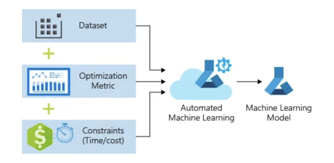
Learn how to automatically generate a regression model to predict taxi fare prices using Azure Machine Learning’s automated machine learning capabilities. The process also involves launching automated machine learning to handle algorithm selection and hyperparameter tuning. Azure ML iterates through various combinations of algorithms and hyperparameters to identify the best model based on your defined criteria.

Contents

• Auto-train a regression model
• Run the model locally with custom parameters
• Explore your model results

1. Auto-train a Regression Model

For this blog, already download the data from Azure Open Datasets and follow the data preparation steps for the NYC Taxi data, as outlined in this tutorial, to make it ready for building your machine learning model.

Configure Workspace

Start by creating workspace object from the existing workspace. A Workspace is a class that accepts your Azure subscription and resource information. It also creates a cloud resource to monitor and track your model runs. Specifically, Workspace.from_config() reads the file config.json and loads the authentication details into an object named ws.

ws is used throughout the rest of the code in this tutorial:

from azureml.core.workspace import Workspace
ws = Workspace.from_config()

Split the Data into Train and Test Sets

To start, split the data into training and test sets using the train_test_split function from the sklearn library. This function divides the data into x, the features dataset for model training, and y, the values to predict, which will be used for testing. The test_size parameter determines the percentage of data allocated to testing, while random_state sets a seed for the random generator, ensuring deterministic splits.

from sklearn.model_selection import train_test_split

x_df = dflow_X.to_pandas_dataframe()
y_df = dflow_y.to_pandas_dataframe()

x_train, x_test, y_train, y_test = train_test_split(x_df, y_df, test_size=0.2, random_state=223)
# flatten y_train to 1d array
y_train.values.flatten()

The purpose of this step is to have data points that weren’t used during training to test the model, allowing us to measure its true accuracy.

2. Run the Model Locally with Custom Parameters

To automatically train a model, follow these steps:

Define Settings for the Experiment Run

• Attach your training data to the configuration and modify settings that control the training process.
• Then, submit the experiment for model tuning. The experiment iterates over different machine learning algorithms and hyperparameter settings, optimizing the accuracy metric to find the best-fit model.

Define Settings for Auto-generation and Tuning

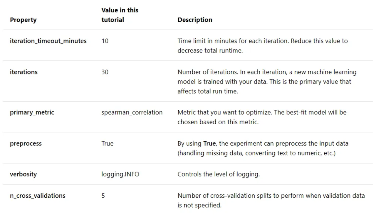
Submitting the experiment with these default settings will take approximately 10–15 min, but if you want a shorter run time, reduce either iterations or iteration_timeout_minutes. Use your defined training settings as a parameter to an AutoMLConfig object.

Use your defined training settings as a parameter to an AutoMLConfig object. Additionally, specify your training data and the type of model, which is regression in this case:

automl_settings = {
    "iteration_timeout_minutes" : 10,
    "iterations" : 30,
    "primary_metric" : 'spearman_correlation',
    "preprocess" : True,
    "verbosity" : logging.INFO,
    "n_cross_validations": 5
}

from azureml.train.automl import AutoMLConfig

# local compute
automated_ml_config = AutoMLConfig(task = 'regression',
                             debug_log = 'automated_ml_errors.log',
                             path = project_folder,
                             X = x_train.values,
                             y = y_train.values.flatten(),
                             **automl_settings)

Train the Automatic Regression Model

To start the experiment locally, pass the automated_ml_config object to the experiment and set show_output=True to view live progress:

from azureml.core.experiment import Experiment
experiment = Experiment(ws, experiment_name)
local_run = experiment.submit(automated_ml_config, show_output=True)

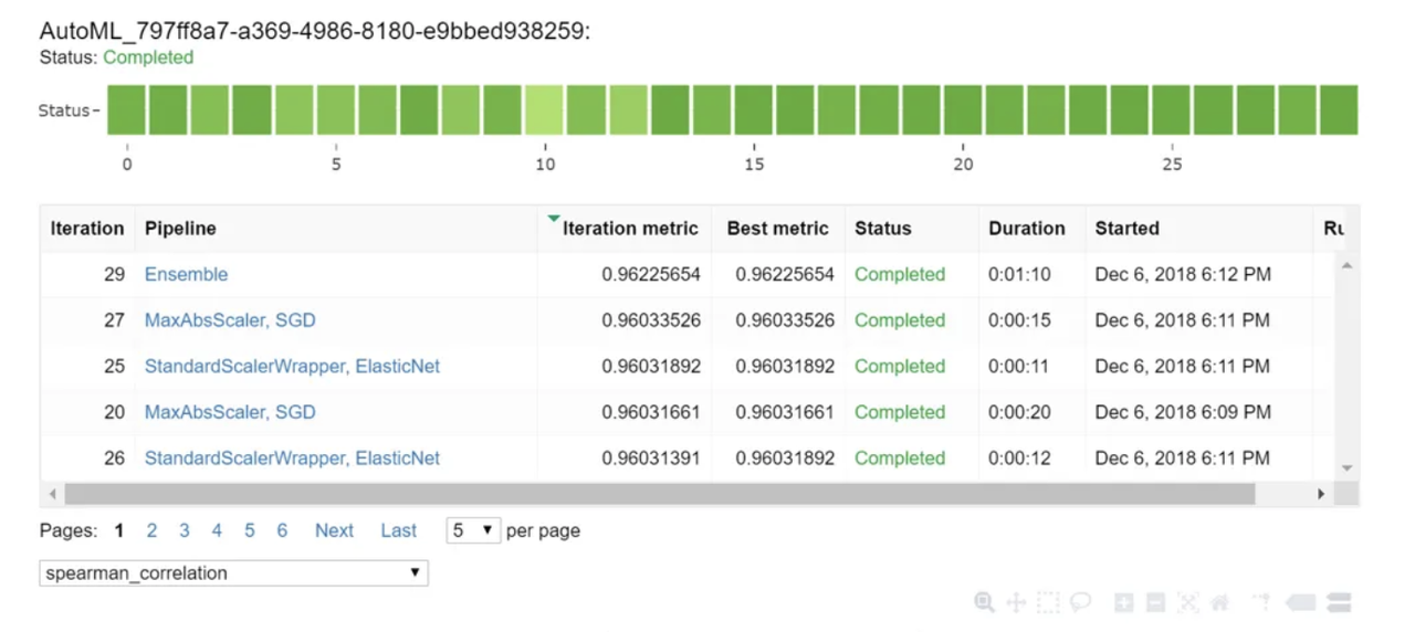
As the experiment runs, you will see the model type, run duration, and training accuracy for each iteration. The “BEST” field tracks the best training score based on the chosen metric.

3. Explore Your Model Results

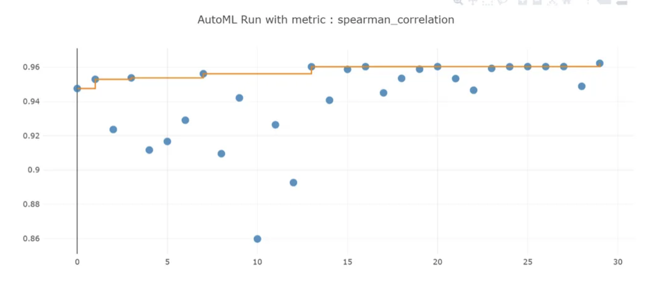
At this point, you can explore the results of the automatic training process using a Jupyter widget or by examining the experiment history. For example, with a Jupyter notebook, you can use this widget to view a graph and a table of results:

from azureml.widgets import RunDetails
RunDetails(local_run).show()

Retrieve the Best Model

Select the best pipeline from the iterations. Use the get_output method to retrieve the best run and fitted model:

best_run, fitted_model = local_run.get_output()
print(best_run)
print(fitted_model)

Test the Best Model Accuracy

To test the model’s accuracy, use the best model to predict taxi fares from the test dataset. Print the first 10 predicted values:

y_predict = fitted_model.predict(x_test.values)
print(y_predict[:10])

To calculate the root mean squared error (RMSE), compare the predicted values to the actual values (y_test):

from sklearn.metrics import mean_squared_error
from math import sqrt

rmse = sqrt(mean_squared_error(y_test, y_predict))
rmse

The result will indicate how far the predicted taxi fare prices are from the actual values. A lower RMSE suggests a better model. The rmse result is 3.2204936862688798.

The traditional machine learning model development process is resource-intensive and time-consuming. Automated machine learning simplifies this by allowing you to rapidly test multiple models for your scenario.

Resources

• Learn more about Azure Machine Learning service
• Learn more about automated machine learning
• Learn more about NYC Taxi data cleaning and preparation